8. Function

Functions are specified using *Function. Each function must have a unique name, and duplicate names are not allowed. *Function is used for time functions or for functions such as failure envelopes in material models.

*Function

Define function

*Function, Type=type, UnitSystem=unitSystem, Name=name
  data line...

Keyword line

• TYPE=type: type of function
  • MultiLinear: Multi-linear function
  • TimeSignal: Time signal. Multi-linear function with fixed step size
  • String: function by mathematical expression
  • HognestadCEnv: Hognestad concrete compressive envelope
  • FIBCEnv: FIB concrete compressive envelope
  • MPPCEnv: Mander-Priestley-Park concrete compressive envelope
  • MPPCIE: Mander-Priestley-Park concrete compressive inelastic strain
  • MaekawaTEnv: Maekawa concrete tensile envelope
• UnitSystem=unitSystem: Local UnitSystem in which the function is defined. It shall be specified in the four-field format force-length-time-temperature. It may be used only when *Environment, TYPE=UnitSystem is defined. If omitted, it is taken to be the same as the global UnitSystem.
• Name=name: function name

Function-related commands define functions in the form of \(\small y=f(x)\) or \(\small y1=f1(x), y2=f2(x), ...\). Functions are used to define envelopes when specifying material models or as time histories when defining loads.

*Function, Type=MultiLinear

Multilinear function

*Function, Type=MultiLinear, Name=name
 x, y1, y2, ..., yn
 ...

First data line and subsequent data lines

• x, y1, y2, ..., yn: Enter values in the form (x, y1, y2, ..., yn).

The MultiLinear function defines the functions y1(x), y2(x), ... in the form of (x, y1(x), y2(x), ..., yn(x)).

Example

*Function, Type=MultiLinear, Name=func1
 0., 45.3
 2.802903E-3, 86.4
 7.26864E-5, 122.5

*Function, Type=MultiLinear, UnitSystem=kN-mm-s-K, Name=func2
 0., 45.3, 12.3
 2.802903E-3, 86.4, 5.1
 7.26864E-5, 122.5, 3.1

*Function, Type=TimeSignal

Time signal. Multi-linear function with fixed step size

*Function, Type=TimeSignal, UnitSystem=unitSystem, Name=name
 dtime, ntime
 file, nseries, scaleFactor, skipRows
 ...

First data line

• dtime: time step (required).
• ntime: number of time data (optional). If the number of rows in the read data exceeds ntime, the extra rows are ignored. If it is less than ntime, the remaining values are padded with zeros. If ntime is not specified, it is automatically set to the length of the longest time series. Other time series shorter than ntime are padded with zeros up to ntime.

Second data line and subsequent data lines

• file: File to be read (required). A text file with values separated by commas, spaces, etc., or an npy file.
• nseries: Number of time series in the file (optional, default 1). For npy files, the number of columns must be the same.
• scale: Scale factor (optional, default 1).
• skipRows: Number of rows to skip at the beginning of the file (optional, default 0). Ignored for npy files.

The TimeSignal function, suitable for representing time histories, can be understood as a multi-linear function with fixed interval x values. The data from the file is read with values separated by whitespace (colon, space, tab, newline). Each file consists of nseries time series data. It reads ntime entries for each of the nseries data. If the file has fewer data entries, the missing values are filled with zeros. At time 0, the value is assumed to be 0, and the first value given in the data corresponds to the value at time dt. The final value corresponds to the value at time ntime*dt.

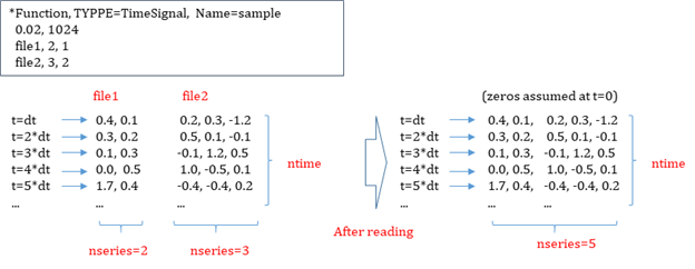
Fig. 8.2-1. TimeSignal function

In the time data file, any content after # is ignored (comment).

Example

*Function, TYPE=TimeSignal, UnitSystem=N-m-s-K, Name=EqAcc
 0.02, 1024              # dt, ntime
 elcenX.dat, 1, 3.01      # file, nseries, scaleFactor
 elcenYZ.dat, 2, 3.01, 4      # dataFile, nseries, scaleFactor, skipRows

*Function, Type=String

Define function by mathematical expression

*Function, Type=STRING, UnitSystem=unitSystem, Name=name
  expression, min,max

First data line

• expression: Expression with x independent variable, such as "sin(x)+1". Note that white space is not allowed.
• min,max: minimum and maximum range. Zero function value is assumed beyond the given range. If Range keyword is not given, no range check is performed

'*Function, TYPE=String' has the feature of parsing the expression. The internal parser supports typical mathematical functions, such as sin(x), cos(x), tan(x), acos(x), atan(x), cosh(x), sinh(x), tanh(x), fabs(x), exp(x), log(x), log10(x), sqrt(x), step(x), sgn(x), and pow(x,n).

Example

*Function, Type=String, Name=Half-sine
 sin(2*pi/1.2*x), 0., 0.6

*Function, Type=HognestadCEnv

Define the compressive envelope of concrete based on Hognestad's curve.

*Function, Type=HognestadCEnv, Name=name
  fco, Ec, ec20, ecu

First data line

• fco: compressive strength (required)
• Ec: initial tangent modulus (required)
• ec20: strain at 0.85fcm concrete stress of descending branch(optional, default 0.003)
• ecu: ultimate strain (optional, always set to max(ec20, ecu) )

Hognestad’s compressive envelope of concrete given as

\[ \small \begin{aligned} & f_c = f_{co} \left[ 2 \frac{\epsilon_c}{\epsilon_{co}} - (\frac{\epsilon_c}{\epsilon_{co}}) ^2 \right], ~~{\rm for}~ \epsilon \le \epsilon_{co}\\ & f_c = f_{co} -0.15 f_{co} \frac{\epsilon - \epsilon_{co}}{\epsilon_{20}-\epsilon_{co}}, ~~{\rm for}~ \epsilon_{co} \lt \epsilon_{c} \le \epsilon_{20} \\ & f_c =0.85 f_{co},~~{\rm for}~ \epsilon_{20} \lt \epsilon_{c} \le \epsilon_{cu} \\ \end{aligned} \]

where, \(\small\epsilon_{20}\) corresponding to \(\small f_{co}\) is given as

\[ \small \epsilon_{co} = 2f_{co} / E_c \]

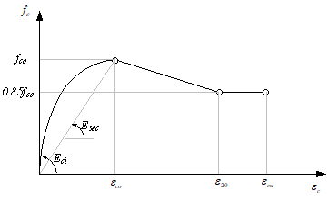
Fig. 8.2-2. Compressive failure envelope of Hognestad model

Example

*Function, Type=HognestadCEnv, Name=HognestadTest1
 25., 23500.

*Function, Type=HognestadCEnv, UnitSystem=kN-mm-s-K, Name=HognestadTest2
 25., 23500., 0.0031, 0.0032

*Function, Type=HognestadCEnv, Name=HognestadTest3
 25., 23500., 0.0032

*Function, Type=ParabolaCEnv

Define the stress-strain compressive envelope for cross-sectional design as specified by EC2 and KDS.

*Function, Type=ParabolaCEnv, UnitSystem=unitSystem, Name=name
  fco, n, eco, ecu

First data line

• fco: design compressive strength, (required)
• n: shape factor (required)
• eco: peak strain (optional, 0.002)
• ecu: ultimate strain (optional, always set to max(eco, ecu) )

The curve given as

\[ \small \begin{aligned} & f_c = f_{co} \left[ 1-(1- \frac{\epsilon_c}{\epsilon_{co}})^n \right], ~~{\textrm for}~ \epsilon \le \epsilon_{co}\\ & f_c = f_{co} ,~~{\textrm for}~ \epsilon_{co} \lt \epsilon_{c} \le \epsilon_{cu} \\ \end{aligned} \]

where, \(\small f_{co} = \phi_c (0.85f_{ck})\), \(\small\phi_c = 0.65\) for ultimate limit state. \(\small\phi_c = 1\) for extreme limit state.

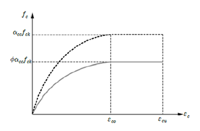
Fig. 8.2-3. ParabolaCEnv function

The elastic modulus, which is the tangent slope, is calculated as follows.

\[ \small E_c = \frac{df}{d\epsilon_c} = f_{co} (1-\frac{\epsilon_c} {\epsilon_{co}})^{n-1} \frac{n}{\epsilon_{co}} \]

Example

*Function, Type=ParabolaCEnv, Name=ParabolaTest1
  0.85*27, 1.8, 0.00203, 0.0033     #  fco, n, eco, ecu

*Function, Type=FIBCEnv

Define the compressive envelope of concrete according to CEB/FIB MC90.

*Function, Type=FIBCEnv, UnitSystem=unitSystem, Name=name
 fcm, Ec, eco

First data line

• fcm: compressive strength (required)
• Ec: initial tangent modulus (required)
• eco: strain at peak concrete strength (optional, default automatically computed)

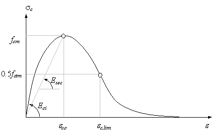
Fig. 8.2-4. Compressive Failure Envelope of EB-FIP MC90

Example

*Function, Type=FIBCEnv, Name=FIBCEnvTest1
 25., 23500.   #  fcm, Ec, eco

*Function, Type=FIBCEnv, Name=FIBCEnvTest2
 25., 23500., 0.002     #  fcm, Ec, eco

*Function, Type=MPPCEnv

Define the compressive envelope of concrete based on the Mander, Priestley, and Park model.

*Function, Type=MPPCEnv Name=name
  fco, Ec, eco, ecu, fcc, esp

First data line

• fco: unconfined compressive strength (required)
• Ec: initial tangent modulus (required)
• eco: strain at peak strength of unconfined concrete (optional, default 0.002)
• ecu: ultimate strain (optional, default 2*eco)
• fcc: confined compressive strength. (optional, default fco)
• esp: spalling strain (optional, default ecu). A straight line is assumed if esp is greater than ecu.

The Mander-Priestley-Park model can define both the confined and unconfined concrete model.

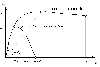
Fig. 8.2-5. Compressive Failure Envelope of Mander, Priestley, Park’s Concrete Model

Example

*Function, Type=MPPCEnv, Name=MPPCEnvTest1
 25., 23500.   #   fco, Ec, eco, ecu, fcc, esp

*Function, Type=MPPCEnv, Name=MPPCEnvTest2
 25., 23500., 0.002, 0.004, 40., 0.006    #   fco, Ec, eco, ecu, fcc, esp

*Function, Type=MPPCIE

Define the inelastic strain of concrete based on the Mander, Priestley, and Park model.

*Function, Type=MPPCIE, UnitSystem=unitSystem, Name=cover
  compressiveEnv, epeak

First data line

• compressiveEnv: Compressive envelope function
• epeak: strain at peak concrete strength (optional, default 0.002). If the given compressiveEnv is a type of MPPCEnv, Hognestad, and CEBFIB, epeak is neglected (automatically computed).

Although this function defines the inelastic strain by the Mander-Priestley-Park model, it can be used with the arbitrary compressive envelope function

Example

*Function, Type=MPPCEnv, Name=concC
 25., 23500.

*Function, Type=MPPCIE, Name=concCI
 concC

*Function, Type=MaekawaTEnv

Maekawa concrete tensile envelope

*Function, Type=MaekawaTEnv, UnitSystem=unitSystem, Name=coverTension
  compressiveEnv,ft, c

First data line

• compressiveEnv: Compressive envelope function(required)
• ft: tensile strength(required)
• c: parameter for Maekawa model (optional, default 0.4)

Maekawa et al. (2002) proposed the following tension softening curve for both normal concrete and reinforced concrete considering tensile hardening, using the same equation:

\[ \small \sigma = f_t \left(\frac{\epsilon_{tu}} {\epsilon_t} \right)^c \]

Here, \(c\) is the factor that determines the shape of the curve. For normal concrete, it should be determined by the following equation based on fracture energy and the characteristic length of the element:

\[ \small \int \sigma_t d \epsilon_t = \int f_t \left(\frac{\epsilon_{tu}} {\epsilon_t} \right)^c d \epsilon_t = \frac {G_F}{l_r} \]

In reinforced concrete, parameter analysis suggests a value of 0.4 for deformed bars and 0.2 for welded wire mesh. Figure 8.2-5 shows a representative result.

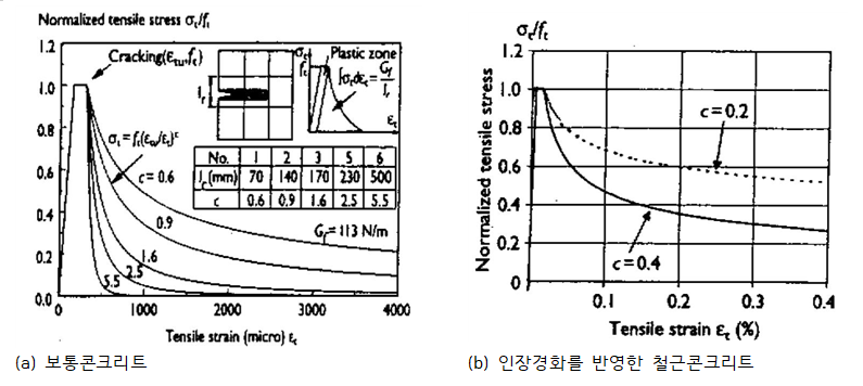
Fig. 8.2-6. Tensile Failure Envelope of Maekawa model

Example

*Function, Type=MPPCEnv, Name=concC
 25, 23500.

*Function, Type=MaekawaTEnv, Name=concT
 concC, 3