7. Material

The material model is specified using *Material. It must have a unique name, and duplicate names cannot be assigned.

*Material

Define material

*Material, TYPE=type, Name=name
 ...datalines depdending type

Keyword line

• TYPE=type: type of materis.

  • __IsoElasticity:__Isotropic Linear Elastic Material
  • OrthoElasticity: Orthotropic Linear Elastic Material
  • vonMises: von Mises plasticity
  • Tresca: Tresca plasticity
  • MohrCoulomb: Mohr-Coulomb plasticity
  • DruckerPrager: Drucker-Prager plasticity
  • ConcreteDamage: Concrete damage plasticity

• Name=name: material name

*Material Type=IsoElasticity

Define isotropic elasticity material

*Material, Type=IsoElasticity, Name=name
 E, nu, alpha, density

First dataline

• E: elastic modulus (required)
• nu: Poisson’s ratio (optional, default 0.)
• alpha: themal expansion coefficient (optional, default 0.)
• density: density (optional, default 0.)

Example

*Material, Type=IsoElasticity Name=iso
 200., 0.2        # E, nu, alpha, density

*Material Type=OrthoElasticity

Define orthotropic elasticity

*Material, Type=OrthoElasticity, Name=name
  E1,E2,E3, G12,G23,G31, nu12,nu23,nu31, a1,a2,a3, density, angle, cs

First dataline

• E1, E2, E3: Elastic moduli(required)
• G12, G23, G31: Shear moduli (required)
• nu12, nu23, nu31: Poison's ratios(required)
• a1,a2,a3: thermal expansion coefficient (optional, default 0)
• density: density(optional, default 0.)
• angle: angle in laminar condition for *Section, TYPE=CompositeShell (optional, default 0.)
• cs: material coodinate system(optional). If not given, global coordinate system is used for material coordinates

Angle is the angle used to define the local coordinate system in the laminar stress condition when defining *Section, TYPE=CompositeShell. CS is used for all other stress conditions.

Example

*Material, Type=OrthoElasticity Name=ortho
 200.,100.,100., 50.,30.,30., 0.12, 0.12, 0.12, 1E-6, 1.2E-6, 1.4E-4, 7810., 0, cs
# E1, E2, E3, G12, G23, G31, nu12, nu23, nu31, a1, a2, a3, density, angle, cs

*Material, Type=OrthoElasticity Name=ortho
 200.,100.,100., 50.,30.,30., 0.12, 0.12, 0.12, 1E-6, 1.2E-6, 1.4E-4, 7810., 90
# E1, E2, E3, G12, G23, G31, nu12, nu23, nu31, a1, a2, a3, density, angle, cs

*Material Type=vonMises

Define von Mises plasticity(J2 plasticity)

*Material, Type=vonMises, Name=name
 E, nu, alpha, density
 yield, H, theta, Kinf, K0, delta

*Material, Type=vonMises, Name=name
 E, nu, alpha, density
 isoHardFunc, kinHardFunc|H

First dataline

• E: elastic modulus (required)
• nu: Poisson’s ratio (optional, default 0.)
• alpha: themal expansion coefficient (optional, default 0.)
• density: density (optional, default 0.)

Second dataline for value (when the first entry is not a function name)

• yield: Initial yield value (required)
• H: slope after initial yield (optional, default 0)
• theta: Mixed hardening parameter (optional, default 0)
• Kinf: Saturation hardening시의 파라미터(optional, default 0)
• K0: Saturation hardening시의 파라미터(optional, default 0)
• delta: Saturation hardening시의 파라미터(optional, default 0)

Second dataline for function (when the first entry is a function name)

• isoHardFunc: Isotropic hardening function. (required)
• kinHardFunc or H: Kinematic hardening function or modulus(optional, default 0)

Value로 지정하는 경우

When specified as Value, the following equation is applied.

• Linear mixed hardening model

\[ \small \begin{aligned} &K(\kappa) = \sigma_Y + \theta \bar{H} \kappa \\ &H'(\kappa) = (1-\theta) \bar{H}, ~ {\rm where,~} 0 \le \theta \le 1 \\ \end{aligned} \]

• Saturation isotropic hardening and linear kinematic hardening model

\[ \small \begin{aligned} &K(\kappa) = \sigma_Y + \theta \bar{H} \kappa + ( \bar{K}_\infty- \bar{K}_0 )(1-exp(-\delta \kappa)) \\ &H'(\kappa) = (1-\theta) \bar{H}, ~ {\rm where,~} 0 \le \theta \le 1 \\ \end{aligned} \]

\(\small\bar{H}\) is a constant, and when \(\small\theta = 0\), only kinematic hardening is applied, while when \(\small\theta = 1\), only isotropic hardening is applied. The condition \(\small 0 \le \theta \le 1\) must be satisfied. In the linear mixed hardening model, \(\small dK/d \kappa = (1-\theta)\bar{H}\) represents the isotropic hardening modulus, and \(\small (1-\theta) \bar{H}\) is the kinematic hardening modulus.

If the conditions \(\small\bar{K}_\infty = \bar{K}_0\) or \(\small\delta = 0\) are satisfied, it corresponds to linear mixed hardening. In linear mixed hardening, \(\bar{H}\) can take negative values; however, in the saturation isotropic hardening and linear kinematic hardening model, the conditions \(\small\bar{H} \ge 0\), \(\small\bar{K}_\infty \ge \bar{K}_0 \gt 0\), and \(\small\delta \ge 0\) must be satisfied.

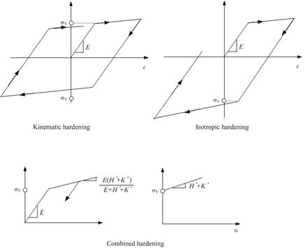
Fig. 7.2-1. Linear hardening

Function으로 지정하는 경우

If uniaxial tensile test results for the material are available, proper calibration can be performed using them. In this case, the appropriate use of Type=Function can be applied. One important point to note is that when both isotropic hardening and kinematic hardening are present, the second elastic modulus must be configured to satisfy the equation as shown in Figure 7.2-2.

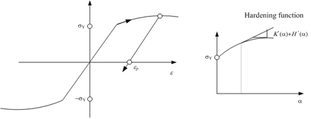
Fig. 7.2-2. Nonlinear hardening

Example

# Linear isotropic hardening case
*Material, Type=vonMises, Name=steel1
 2000000.          # E, nu, alpha, density
 3000., 300.,1.    # yield, H, theta, Kinf, K0, delta

# Linear kinematic hardening case
*Material, Type=vonMises, Name=steel2
 2000000.        # E, nu, alpha, density
 3000., 300.,    # yield, H, theta, Kinf, K0, delta

# Nonlinear isotropic hardening case
*Function, Type=MultiLinear, Name=isoFunc 
 0. 200.
 0.01 210.

*Material, Type=vonMises, Name=steel3
 200000.    # E, nu, alpha, density
 isoFunc    # isoHardFunc, kinHardFunc|H

# Nonlinear isotropic hardening, linear kinematic hardneing case
*Material, Type=vonMises, Name=steel4
 200000.    # E, nu, alpha, density
 isoFunc, 20.      # isoHardFunc, kinHardFunc|H

# Nonlinear isotropic/kinematic hardneing case
*Material, Type=vonMises, Name=steel5
 200000.    # E, nu, alpha, density
 isoFunc, kinFunc     # isoHardFunc, kinHardFunc|H

*Material Type=Tresca

Define Tresca plasticity material model

*Material, Type=Tresca, Name=name
 E, nu, alpha, density, StrainHardening|IsotropicHardening
 {yield,dyield}|yieldFunc

First dataline

• E: elastic modulus (required)
• nu: Poisson’s ratio (optional, default 0.)
• alpha: themal expansion coefficient (optional, default 0.)
• density: density (optional, default 0.)
• StrainHardening|IsotropicHardening: hardening type(optional, default “StrainHardening”)

Second dataline

• yield,dyield: initial yield value(required), and the derivative after initial yielding(optional, default 0.)
• yieldFunc: yield function(required)

The Tresca material model has the following yield function and flow potential:

\[ \small F({\sigma}, \kappa) = | \sigma_1 - \sigma_3 | - \sigma_Y (\kappa) \]

The hardening rule can apply strain hardening, work hardening, or the isotropic associative hardening rule. In the Tresca model, work hardening and associative isotropic hardening are identical.

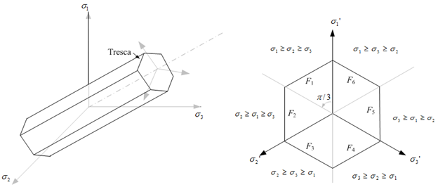
Fig. 7.2-3. Tresca yield criteria

Example

*Function, Type=MultiLinear, Name=trYield
 0. 0.
 0.01 10.
 0.02  15

# no hardening case with sy = 20. 
*Material, Type=Tresca, Name=steelT1
 2E6, 0.18, 1E-5, 7850   # E, nu, alpha, density
 20                      # yield, dyield

# linear hardening case with strain hardening 
*Material, Type=Tresca, Name=steelT2
 2E6, 0.18, 1E-5, 7850   # E, nu, alpha, density
 20, 0.1                 # yield, dyield

# linear hardening case with work hardening
*Material, Type=Tresca, Name=steelT3
 2E6, 0.18, 1E-5, 7850                    # E, nu, alpha, density
 20, 0.1, StrainHardening|WorkHardening   # yield, dyield, StrainHardening|WorkHardening

# nonlinear hardening case with work hardening
*Material, Type=Tresca, Name=steelT4
 2E6, 0.18, 1E-5, 7850   # E, nu, alpha, density
 trYield                 # yieldFunc

*Material Type=MohrCoulomb

Define Mohr-Coulomb material

*Material, Type=MohrCoulomb, Name=name
 E, nu, alpha, density, StrainHardening|IsotropicHardening
 {coh,dcoh}|cohFunc
 {fric,dfric}|fricFunc 
 {dila,ddila}|dilaFunc   

First dataline

• E: elastic modulus (required)
• nu: Poisson’s ratio (optional, default 0.)
• alpha: themal expansion coefficient (optional, default 0.)
• density: density (optional, default 0.)
• StrainHardening|IsotropicHardening: hardening type(optional, default “StrainHardening”)

Second dataline

• coh,dcoh: initial value (required) and derivative of cohesion (optional, default 0.)
• cohFunc: function name of cohesion function (required)

Third dataline (frictional quatities)

• fric,dfric: initial value(required) and derivative of friction angle. (optional, default 0.)
• fricFunc: function name of friction angle function (required)

Forth dataline (dilatent quanties)

• dila,ddila: initial value and derivative of dilatent angle (default 0., 0.)
• dilaFunc: function name of dilatent function (optional)

The units for the frictional angle and dilatant angle are in degrees, not radians. If the value of the dilatant angle is equal to the frictional angle, the associative flow rule is applied. Otherwise, the non-associative flow rule is applied. The initial cohesion (cohesion0) must be specified as a non-zero value. When using the associative isotropic hardening (i.e., IsotropicHardening) as the hardening rule, constant frictional and dilatant angles must be used.

The Mohr-Coulomb material model uses the following yield function and plastic potential.

\[ \small F( \sigma, \kappa) = (\sigma_1 - \sigma_3) +(\sigma_1+\sigma_3) \sin \phi - 2 c(\kappa) \cos(\phi(\kappa)) \]

\[ \small G( \sigma, \kappa) = (\sigma_1 - \sigma_3) +(\sigma_1+\sigma_3) \sin \psi - 2 c(\kappa) \cos(\psi(\kappa)) \]

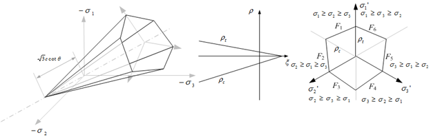
Fig. 7.2-4. Mohr-Coulomb yield criteria

경화법칙은 strain hardening과 isotropic hardening이 존재한다. Mohr-Coulomb 모델에서는 work hardening이 존재하지 않는다.

Example

# associative flow rule, no hardening
*Material, TYPE=MohrCoulomb, Name=soil1
 2E6, 0.18, 1E-5, 7850
 20    # coh, dcoh 
 35    # fric, dfric
 35    # dila, ddila

# associative flow rule, strain hardening
# linear hardening of cohesion, constant friction and dilatency
*Material, TYPE=MohrCoulomb, Name=soil2
 2E6, 0.18, 1E-5, 7850
 20,3. 
 35, 
 30. 

# associative flow rule, associative isotropic hardening
# linear hardening of cohesion, constant friction and dilatency
*Material, TYPE=MohrCoulomb, Name=soil3
 2E6, 0.18, 1E-5, 7850, IsotropicHardening
 20,3. 
 35, 
 30. 

# associative flow rule, associative isotropic hardening,
# linear hardening of cohesion, friction
*Material, TYPE=MohrCoulomb, Name=soil4
 2E6, 0.18, 1E-5, 7850
 20,3. 
 35, 0.2 
 35, 0.2 

# non-associative flow rule, strain hardening, 
# nonlinear hardening of cohesion, friction, dilatency
*Function, Name=cohFunc
 0., 20.
 0.001, 25.
 0.002, 25.

*Function, Name=fricFunc
 0. 35.
 0.001, 40.
 0.002, 45.

*Function, Name=dilaFunc
 0. 30.
 0.001 35.
 0.002 40.

*Material, TYPE=MohrCoulomb, Name=soil5
 2E6, 0.18, 1E-5, 7850
 cohFunc 
 fricFunc
 dilaFunc

*Material Type=DruckerPrager

Define Isotropic elasticity material

*Material, Type=DruckerPrager, Name=name
 E, nu, alpha, density, StrainHardening|IsotropicHardening
 beta
 coh,dcoh|cohFunc, 
 af,daf|afFunc 
 ap,dap|apFunc  

First dataline

• E: elastic modulus (required)
• nu: Poisson’s ratio (optional, default 0.)
• alpha: themal expansion coefficient (optional, default 0.)
• density: density (optional, default 0.)
• StrainHardening|IsotropicHardening: hardening type(optional, default “StrainHardening”)

Second dataline

• beta: beta (required)

3rd dataline

• coh, dcoh: initial value(required) and derivative of cohesion (optional, default 0.,0.)
• cohFunc: function name of cohesion(required)

4th dataline (frictional quantity)

• af, daf: initial value and derivative of alpha. ( default 0., 0.)
• afFunc: function name of alpha (required)

5th dataline (dilatent quantity)

• ap, dap: initial value(required) and derivative of alphaP (dilatency) (optional, default 0.)
• apFunc: function name of alphaP (required)

The units for the frictional angle and dilatant angle are in degrees, not radians. If the value of the dilatant angle is equal to the frictional angle, the associative flow rule is applied. Otherwise, the non-associative flow rule is applied. The initial cohesion (cohesion0) must be specified as a non-zero value. When using the associative isotropic hardening (i.e., IsotropicHardening) as the hardening rule, constant frictional and dilatant angles must be used.

In the Drucker-Prager material model, the yield function and plastic potential are as follows.

\[ \small F( \sigma, \kappa) = || s || + \alpha (\kappa) I_1 - \beta c(\kappa) \]

▪ Flow potential : same to yield function

\[ \small G( \sigma, \kappa) = || s || + \alpha_p (\kappa) I_1 \]

경화법칙은 strain hardening과 isotropic hardening이 존재한다. Drucker-Prager 모델에서는 work hardening이 존재하지 않는다.

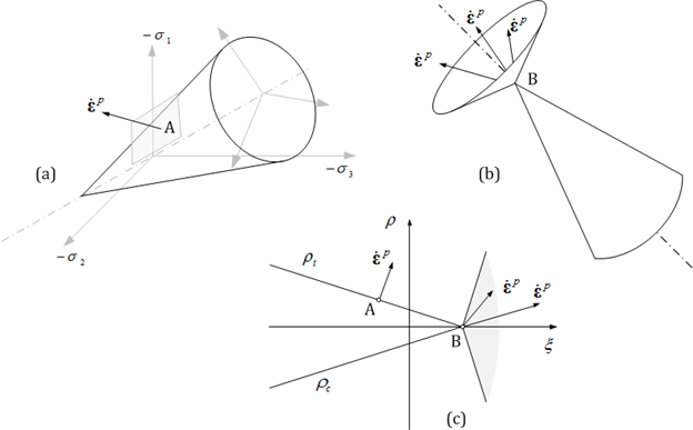
Fig. 7.2-5. Flow rule of Drucker-Prager model

Example

*Material, TYPE=DruckerPrager, Name=concreteDP
 2E6, 0.18, 1E-5, 7850, StrainHardening   # E, nu, alpha, density, StrainHardening|IsotropicHardening
 4        # beta
 12.3     # coh,dcoh|cohFunc, 
 20       # af,daf|afFunc 
 20       # ap,dap|apFunc  

*Material Type=ConcreteDamage

Define concrete damage plasticity

*Material, Type=ConcreteDamage, Name=name
 E, nu, alpha, density
 fc, Dc, wc, 
 ft, Dt, wt, 
 a, Kc, ap,ecc 

First dataline

• E: elastic modulus (required)
• nu: Poisson’s ratio (optional, default 0.)
• alpha: themal expansion coefficient (optional, default 0.)
• density: density (optional, default 0.)

Second dataline

• fc,Dc,wc: compressive uniaxial yield function(required), damage function(option, default none), and recovery(optional, default 0.)

3rd dataline

• ft,Dt,wt: tensile uniaxial yield function(required), damage function(option, default none), and recovery(optional, default 0.)

4th dataline if necessary (parameters for yield surface and flow potential)

• a: parameter for yield surface related to biaxial stress condition (optional, default 0.14),
• Kc: parameter for yield surface related to triaxial stress condition (optional, default 2/3),
• ap: parameter for flow potential related to dilatency(optional, default 0.2)
• ecc: parameter for flow potential, the eccentricity(optional, default 0.1)

Example

*Function, Name=chard
 0., 20.
 0.001, 25.
 0.002, 25.

*Function, Name=thard
 0., 2.
 0.001, 1.
 0.002, 0.2. 

*Material, TYPE=ConcreteDamage, Name=concreteCD
 29188.6, 0.18, 2300, 1e-05  #  E, nu, alpha, density
 chard,  , 1  # fc, Dc, wc n thard,  , 1  # ft, Dt, wt
 0.12 , 0.666667, 0.2, 0.1  # a, Kc, ap, ecc

*Material Type=UConcrete

Define uniaxial concrete

*Material, Type=UConrete, Name=name 
  CEnvFunc, Plastic|Secant|CIEFunc, alpha, density, timeProp
  TEnvFunc, Plastic|Secant|TIEFunc 

First dataline

• CEnvFunc: Compressive envelope function (required)
• Plastic|Secant|CIEFunc: - Plastic unloading, Secant unloading, 또는 damage plastic unloading 시의 함수를 지정 (optional, default Plastic)
• alpha: themal expansion coefficient (optional, default 0.)
• density: density (optional, default 0.)
• timeProp: Combined viscosity material given by *Material, Type=UConcreteTime. (optional)

2rd dataline if necessary

• TEnvFunc: Tensile envelope function (optional)
• Plastic|Secant|TIEFunc: - Plastic unloading, Secant unloading, 또는 damage plastic unloading 시의 함수를 지정 (optional, default Secant)
• TIEFunc: Tensile unloading function iff Plasticity (optional)

The UConcrete model is a simplified plastic-damage model that neglects energy dissipation during unloading and reloading in the compressive side of concrete. Independent failure envelopes must be defined for both compression and tension sides, and during unloading/reloading, one can choose between a plastic model without damage (hereafter referred to as plastic), a plastic-damage model (hereafter referred to as damage plastic), or a plastic-elastic model (hereafter referred to as damage elastic). If applying the plastic-damage model, unloading and reloading are carried out along the segment connecting the point corresponding to the most recent strain (\(\small\epsilon_{cun}\) or \(\epsilon_{tun}\) at point \(\small(\epsilon_{cun},\sigma_{cun})\) or \(\small(\epsilon_{tun},\sigma_{tun})\)) and the plastic strain specified by the plastic strain function (corresponding to \(\small\epsilon_{cpl}\) or \(\epsilon_{tpl}\)). Therefore, it is necessary to specify the function in the form of \(\small(\epsilon_{cpl},\sigma_{cun})\) or \(\small(\epsilon_{tpl},\sigma_{tun})\).

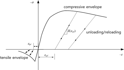
Fig. 7.2-6. Failure envelope, unloading/reloading of UConcrete

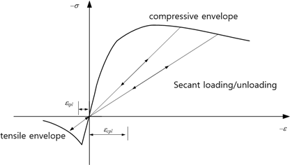
Fig. 7.2-7. Secant unloading/unloading of UConcrete

Under cyclic loading conditions, elastic behavior continues until the yield value corresponding to the plastic strain is reached, after which yielding follows the failure envelope. When secant loading/unloading is specified, there is no corresponding inelastic strain.

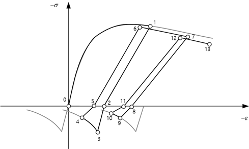
Fig. 7.2-8. Cyclic loading of UConcrete

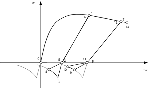
Fig. 7.2-9. Cyclic loading of Unconcret for tensile secant unloading

Example

*Function, Type=MPPCEnv, Name=MPP
 27, 25000, 0.002   # fco, Ec, eco, ecu, fcc, esp

*Function, Type=MPPCIE, Name=MPPIE
 MPP   # compressiveEnv, epeak 

*Function, Type=MaekawaTEnv, Name=Maekawa
 MPP, 3, 0.4  # compressiveEnv,ft, c

*Material, Type=UConcrete, Name=Mander
 MPP, MPPIE
 Maekawa,Secant   

*Material, Type=UConcrete, Name=Mander
 MPP
 Maekawa, Secant

*Material Type=USteel

Define uniaxial steel model based on Menegotto-Pinto model

*Material, Type=USteel, Name=name 
  E0, yield, E1,  R0,a1,a2, a3,a4, eu, alpha, density

First dataline

• E0: Initial tangent modulus (required)
• yield: yield stress ( required )
• E1: Second tangent modulus (optional, default 0.)
• __R0,a1,a2:__curvature parameters (optional, default 20, 0, 0)
• a3,a3: isotropic hardening parameters (optional, default 0, 1.)
• eu: ultimate strain (optional, default 0). If eu = 0., then ultimate strain is not checked.
• alpha: themal expansion coefficient (optional, default 0.)
• density: density (optional, default 0.)

USteel uses Menegotto-Pinto model with some modifications of partial reloading problem. It can be used for modeling rebar or prestressing steel.

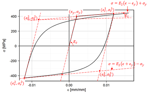
Fig. 7.2-10 Menegotto-Pinto Model

The recommended values of modeling rebar and 7-wire strand is given in the example.

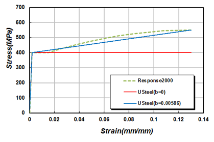
Fig. 7.2-11 Stress-strain curve of a weldable rebar with 400 MPa yield strength

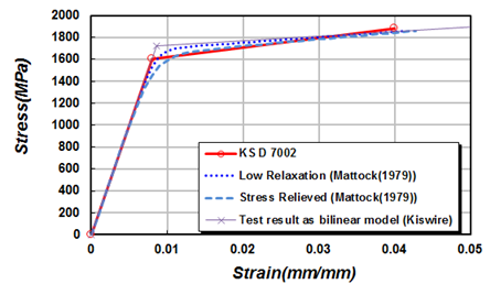
Fig. 7.2-12 Stress-strain curve of 7-wire strand with ultimate strength 1860 MPa

Example

# 400 MPa rebar without hardening
*Material, Type=USteel, Name=SD40
 200000,400, 0, 20,18.5,0.15, 0.01, 7, 0.08
#  E0, yield, E1, R0,a1,a2, a3,a4, eu, alpha, density

# 400 MPa weldable rebar without hardening
*Material, Type=USteel, Name=SD40W
 200000, 400, 0, 20,18.5,0.15, 0.01, 7, 0.13
#  E0, yield, E1, R0,a1,a2, a3,a4, eu, alpha, density

# 400 MPa rebar with hardening
*Material, Type=USteel, Name=SD40-U
 200000, 400, 0.01282*200000, 20,18.5,0.15, 0.01, 7, 0.08

# 400 MPa weldable rebar with hardening
*Material, Type=USteel, Name=SD40W-U
 200000, 400, 0.0586*200000, 20,18.5,0.15, 0.01, 7, 0.13

# Stress-relieved 7-wire strand with ultimate strength 1860 MPa 
*Material, Type=USteel, Name=STendon
 200000,  1652.891, 200000*0.03, 6, 0., 0., 0, 1, 0.0428

# Low relaxation 7-wire strand with ultimate strength 1860 MPa 
*Material, Type=USteel, Name=RTendon
 200000,  1694.915, 200000*0.025, 10,0.,0., 0, 1, 0.0415

*Material Type=GapHook

Specify uniaxial gap-hook material.

*Material, Type=GapHook, Name=name 
  kg,g, kh,h

First dataline

• kg,g: tangent and gap in compression part (optional, default 0.,0.)
• __kh,h:__tangent and hook tension part (optional,default 0.,0.)

Using the GapHook command, you can model tension-only or compression-only behavior. Both kg and kh cannot be zero at the same time.

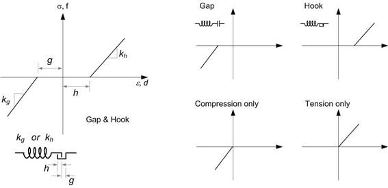
Fig. 7.2-135.GapHook Model

Example

*Material, Type=GapHook, Name=gaphook
 5E5, 0.1, 4E5, 0.2   # kg, g, kh, h

# tension only
*Material, Type=GapHook, Name=cable
 0, 0, 5E5   # kg, g, kh, h

# compression only
*Material, Type=GapHook, Name=contactSpring
 5E5   # kg, g, kh, h

*Material Type=Acoustic

Acoustic solid 요소용 acoustic material을 지정

*Material, Type=Acoustic, Name=name 
  bulk, density

First dataline

• bulk: Bulk modulus (required). If zero bulk moduls is given, the acoustic medium is assumed to be incompressible (Laplace equation is used)
• __density:__density (required)

Example

*Material, Type=Acoustic, Name=water
 2190E6, 1000

*Material Type=Porous

Specify porous material for porous solid elements.

*Material, Type=Acoustic, Name=name 
  solidMat, wBulk, wDen, porosity, perm

First dataline

• solidMat: normal material for solid
• wBulk: bulk modulus of water (required)
• wDensity: water density(required)
• porosity: porosity (required)
• perm: permeability (required)

Example

*Material, Type=Porous, Name=water
 mat, 1000, 100, 0.1, 1000