7. 재료

재료모델은 *Material로 지정한다. 고유이름을 가지며 이름은 중복하여 지정할 수 없다.

*Material

Define material

*Material, TYPE=type, Name=name
 ...datalines depdending type

Keyword line

• TYPE=type: type of materis.

  • __IsoElasticity:__Isotropic Linear Elastic Material
  • OrthoElasticity: Orthotropic Linear Elastic Material
  • vonMises: von Mises plasticity
  • Tresca: Tresca plasticity
  • MohrCoulomb: Mohr-Coulomb plasticity
  • DruckerPrager: Drucker-Prager plasticity
  • ConcreteDamage: Concrete damage plasticity

• Name=name: material name

*Material Type=IsoElasticity

Define isotropic elasticity material

*Material, Type=IsoElasticity, Name=name
 E, nu, alpha, density

First dataline

• E: elastic modulus (required)
• nu: Poisson’s ratio (optional, default 0.)
• alpha: themal expansion coefficient (optional, default 0.)
• density: density (optional, default 0.)

Example

*Material, Type=IsoElasticity Name=iso
 200., 0.2        # E, nu, alpha, density

*Material Type=OrthoElasticity

Define orthotropic elasticity

*Material, Type=OrthoElasticity, Name=name
  E1,E2,E3, G12,G23,G31, nu12,nu23,nu31, a1,a2,a3, density, angle, cs

First dataline

• E1, E2, E3: Elastic moduli(required)
• G12, G23, G31: Shear moduli (required)
• nu12, nu23, nu31: Poison's ratios(required)
• a1,a2,a3: thermal expansion coefficient (optional, default 0)
• density: density(optional, default 0.)
• angle: angle in laminar condition for *Section, TYPE=CompositeShell (optional, default 0.)
• cs: material coodinate system(optional). If not given, global coordinate system is used for material coordinates

angle은 *Section, TPYE=CompositeShell을 정의할 때 사용되는 laminar stress condition에서의 국부 좌표계 정의를 위한 각도이다. cs는 이를 제외한 모든 응력 조건에 사용된다.

Example

*Material, Type=OrthoElasticity Name=ortho
 200.,100.,100., 50.,30.,30., 0.12, 0.12, 0.12, 1E-6, 1.2E-6, 1.4E-4, 7810., 0, cs
# E1, E2, E3, G12, G23, G31, nu12, nu23, nu31, a1, a2, a3, density, angle, cs

*Material, Type=OrthoElasticity Name=ortho
 200.,100.,100., 50.,30.,30., 0.12, 0.12, 0.12, 1E-6, 1.2E-6, 1.4E-4, 7810., 90
# E1, E2, E3, G12, G23, G31, nu12, nu23, nu31, a1, a2, a3, density, angle, cs

*Material Type=vonMises

Define von Mises plasticity(J2 plasticity)

*Material, Type=vonMises, Name=name
 E, nu, alpha, density
 yield, H, theta, Kinf, K0, delta

*Material, Type=vonMises, Name=name
 E, nu, alpha, density
 isoHardFunc, kinHardFunc|H

First dataline

• E: elastic modulus (required)
• nu: Poisson’s ratio (optional, default 0.)
• alpha: themal expansion coefficient (optional, default 0.)
• density: density (optional, default 0.)

Second dataline for value (첫 항이 함수명이 아닌 경우)

• yield: Initial yield value (required)
• H: slope after initial yield (optional, default 0)
• theta: Mixed hardening parameter (optional, default 0)
• Kinf: Saturation hardening시의 파라미터(optional, default 0)
• K0: Saturation hardening시의 파라미터(optional, default 0)
• delta: Saturation hardening시의 파라미터(optional, default 0)

Second dataline for function (첫 항이 함수명인 경우)

• isoHardFunc: Isotropic hardening function. (required)
• kinHardFunc or H: Kinematic hardening function or modulus(optional, default 0)

Value로 지정하는 경우

Value로 지정하는 경우 다음의 수식을 적용한다.

• Linear mixed hardening model

\[ \small \begin{aligned} &K(\kappa) = \sigma_Y + \theta \bar{H} \kappa \\ &H'(\kappa) = (1-\theta) \bar{H}, ~ {\rm where,~} 0 \le \theta \le 1 \\ \end{aligned} \]

• Saturation isotropic hardening and linear kinematic hardening model

\[ \small \begin{aligned} &K(\kappa) = \sigma_Y + \theta \bar{H} \kappa + ( \bar{K}_\infty- \bar{K}_0 )(1-exp(-\delta \kappa)) \\ &H'(\kappa) = (1-\theta) \bar{H}, ~ {\rm where,~} 0 \le \theta \le 1 \\ \end{aligned} \]

\(\small\bar{H}\)는 상수이며, \(\small\theta = 0\)이면 kinematic hardening만을, \(\small\theta = 1\)이면 isotropic hardening만을 적용하는 것이다. \(\small 0 \le \theta \le 1\)의 조건을 만족해야 한다. Linear mixed hardening model에서 \(\small dK/d \kappa = (1-\theta)\bar{H}\) 가 isotropic hardening molulus가 되고, \(\small (1-\theta) \bar{H}\)이 kinematic hardening modulus가 된다.

\(\small\bar{K}_\infty = \bar{K}_0\)또는 \(\small\delta=0\) 조건을 만족할 경우 linear mixed hardening에 해당한다. Linear mixed hardening에서 \(\bar{H}\)는 음의 값을 가질 수 있으나, Saturation isotropic hardening and linear kinematic hardening model에서는 \(\small\bar{H} \ge 0\), \(\small\bar{K}_\infty \ge \bar{K}_0 \gt 0\), \(\small\delta \ge 0\) 조건을 만족해야 한다.

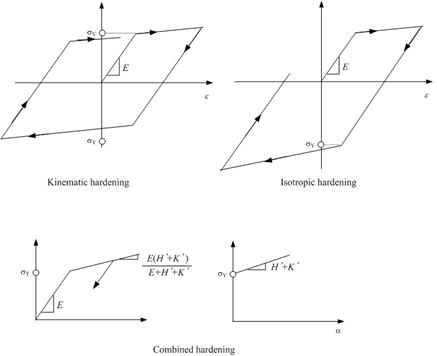
Fig. 7.2-1. Linear hardening

Function으로 지정하는 경우

재료에 대한 1축 인장 실험결과가 있다면, 이를 이용하여 절절히 calibration을 수행할 수 있다. 이 경우 Type=Function을 적절히 이용하면 된다. 주의할 점은 isotropic hardening과 kinematic hardening이 동시에 존재할 때 2차탄성계수 가 그림 7.2-2에 제시된 것과 같은 식을 만족하도록 구성해야 한다는 점이다.

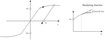
Fig. 7.2-2. Nonlinear hardening

Example

# Linear isotropic hardening case
*Material, Type=vonMises, Name=steel1
 2000000.          # E, nu, alpha, density
 3000., 300.,1.    # yield, H, theta, Kinf, K0, delta

# Linear kinematic hardening case
*Material, Type=vonMises, Name=steel2
 2000000.        # E, nu, alpha, density
 3000., 300.,    # yield, H, theta, Kinf, K0, delta

# Nonlinear isotropic hardening case
*Function, Type=MultiLinear, Name=isoFunc 
 0. 200.
 0.01 210.

*Material, Type=vonMises, Name=steel3
 200000.    # E, nu, alpha, density
 isoFunc    # isoHardFunc, kinHardFunc|H

# Nonlinear isotropic hardening, linear kinematic hardneing case
*Material, Type=vonMises, Name=steel4
 200000.    # E, nu, alpha, density
 isoFunc, 20.      # isoHardFunc, kinHardFunc|H

# Nonlinear isotropic/kinematic hardneing case
*Material, Type=vonMises, Name=steel5
 200000.    # E, nu, alpha, density
 isoFunc, kinFunc     # isoHardFunc, kinHardFunc|H

*Material Type=Tresca

Define Tresca plasticity material model

*Material, Type=Tresca, Name=name
 E, nu, alpha, density, StrainHardening|IsotropicHardening
 {yield,dyield}|yieldFunc

First dataline

• E: elastic modulus (required)
• nu: Poisson’s ratio (optional, default 0.)
• alpha: themal expansion coefficient (optional, default 0.)
• density: density (optional, default 0.)
• StrainHardening|IsotropicHardening: hardening type(optional, default “StrainHardening”)

Second dataline

• yield,dyield: initial yield value(required), and the derivative after initial yielding(optional, default 0.)
• yieldFunc: yield function(required)

Tresca 재료모델은 항복함수와 소성퍼텐션(flow potential)이 다음과 같다.

\[ \small F({\sigma}, \kappa) = | \sigma_1 - \sigma_3 | - \sigma_Y (\kappa) \]

경화법칙(hardening rule)은 strain hardening, work harding, isotropic associative hardening rule이 적용가능한데, Tesca 모델에서는 work hardening과 associative isotropic hardening이 동일하다.

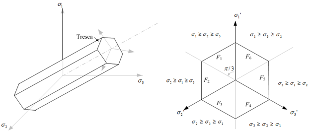
Fig. 7.2-3. Tresca yield criteria

Example

*Function, Type=MultiLinear, Name=trYield
 0. 0.
 0.01 10.
 0.02  15

# no hardening case with sy = 20. 
*Material, Type=Tresca, Name=steelT1
 2E6, 0.18, 1E-5, 7850   # E, nu, alpha, density
 20                      # yield, dyield

# linear hardening case with strain hardening 
*Material, Type=Tresca, Name=steelT2
 2E6, 0.18, 1E-5, 7850   # E, nu, alpha, density
 20, 0.1                 # yield, dyield

# linear hardening case with work hardening
*Material, Type=Tresca, Name=steelT3
 2E6, 0.18, 1E-5, 7850                    # E, nu, alpha, density
 20, 0.1, StrainHardening|WorkHardening   # yield, dyield, StrainHardening|WorkHardening

# nonlinear hardening case with work hardening
*Material, Type=Tresca, Name=steelT4
 2E6, 0.18, 1E-5, 7850   # E, nu, alpha, density
 trYield                 # yieldFunc

*Material Type=MohrCoulomb

Define Mohr-Coulomb material

*Material, Type=MohrCoulomb, Name=name
 E, nu, alpha, density, StrainHardening|IsotropicHardening
 {coh,dcoh}|cohFunc
 {fric,dfric}|fricFunc 
 {dila,ddila}|dilaFunc   

First dataline

• E: elastic modulus (required)
• nu: Poisson’s ratio (optional, default 0.)
• alpha: themal expansion coefficient (optional, default 0.)
• density: density (optional, default 0.)
• StrainHardening|IsotropicHardening: hardening type(optional, default “StrainHardening”)

Second dataline

• coh,dcoh: initial value (required) and derivative of cohesion (optional, default 0.)
• cohFunc: function name of cohesion function (required)

Third dataline (frictional quatities)

• fric,dfric: initial value(required) and derivative of friction angle. (optional, default 0.)
• fricFunc: function name of friction angle function (required)

Forth dataline (dilatent quanties)

• dila,ddila: initial value and derivative of dilatent angle (default 0., 0.)
• dilaFunc: function name of dilatent function (optional)

마찰각(frictional angle) 및 팽창각(dialtent angle)의 단위는 라디안이 아닌 degree가 사용된다. 팽창각 관련 값이 마찰각과 같다면, 연관소성흐름 법칙(associative flow rule)이 적용된다. 그렇지 않으면 비연관소성흐름법칙(non-associative flow rule)이 적용된다. 초기 점착력(cohesion0은 반드시 0이 아닌 값을 지정해야 한다. 경화법칙으로 associative isotropic hardening(즉, IsotropicHardening)을 적용할 때는 일정한 마찰각과 팽창각(constant frictional and dilatent angle)이 사용되어야 한다.

Mohr-Coulomb 재료모델은 다음과 같은 항복함수와 소성퍼텐셜을 사용한다.

\[ \small F( \sigma, \kappa) = (\sigma_1 - \sigma_3) +(\sigma_1+\sigma_3) \sin \phi - 2 c(\kappa) \cos(\phi(\kappa)) \]

\[ \small G( \sigma, \kappa) = (\sigma_1 - \sigma_3) +(\sigma_1+\sigma_3) \sin \psi - 2 c(\kappa) \cos(\psi(\kappa)) \]

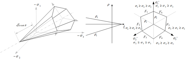
Fig. 7.2-4. Mohr-Coulomb yield criteria

The hardening rule includes strain hardening and isotropic hardening. In the Mohr-Coulomb model, work hardening does not exist.

Example

# associative flow rule, no hardening
*Material, TYPE=MohrCoulomb, Name=soil1
 2E6, 0.18, 1E-5, 7850
 20    # coh, dcoh 
 35    # fric, dfric
 35    # dila, ddila

# associative flow rule, strain hardening
# linear hardening of cohesion, constant friction and dilatency
*Material, TYPE=MohrCoulomb, Name=soil2
 2E6, 0.18, 1E-5, 7850
 20,3. 
 35, 
 30. 

# associative flow rule, associative isotropic hardening
# linear hardening of cohesion, constant friction and dilatency
*Material, TYPE=MohrCoulomb, Name=soil3
 2E6, 0.18, 1E-5, 7850, IsotropicHardening
 20,3. 
 35, 
 30. 

# associative flow rule, associative isotropic hardening,
# linear hardening of cohesion, friction
*Material, TYPE=MohrCoulomb, Name=soil4
 2E6, 0.18, 1E-5, 7850
 20,3. 
 35, 0.2 
 35, 0.2 

# non-associative flow rule, strain hardening, 
# nonlinear hardening of cohesion, friction, dilatency
*Function, Name=cohFunc
 0., 20.
 0.001, 25.
 0.002, 25.

*Function, Name=fricFunc
 0. 35.
 0.001, 40.
 0.002, 45.

*Function, Name=dilaFunc
 0. 30.
 0.001 35.
 0.002 40.

*Material, TYPE=MohrCoulomb, Name=soil5
 2E6, 0.18, 1E-5, 7850
 cohFunc 
 fricFunc
 dilaFunc

*Material Type=DruckerPrager

Define Isotropic elasticity material

*Material, Type=DruckerPrager, Name=name
 E, nu, alpha, density, StrainHardening|IsotropicHardening
 beta
 coh,dcoh|cohFunc, 
 af,daf|afFunc 
 ap,dap|apFunc  

First dataline

• E: elastic modulus (required)
• nu: Poisson’s ratio (optional, default 0.)
• alpha: themal expansion coefficient (optional, default 0.)
• density: density (optional, default 0.)
• StrainHardening|IsotropicHardening: hardening type(optional, default “StrainHardening”)

Second dataline

• beta: beta (required)

3rd dataline

• coh, dcoh: initial value(required) and derivative of cohesion (optional, default 0.,0.)
• cohFunc: function name of cohesion(required)

4th dataline (frictional quantity)

• af, daf: initial value and derivative of alpha. ( default 0., 0.)
• afFunc: function name of alpha (required)

5th dataline (dilatent quantity)

• ap, dap: initial value(required) and derivative of alphaP (dilatency) (optional, default 0.)
• apFunc: function name of alphaP (required)

마찰각(frictional angle) 및 팽창각(dialtent angle)의 단위는 라디안이 아닌 degree가 사용된다. 팽창각 관련 값이 마찰각과 같다면, 연관소성흐름 법칙(associative flow rule)이 적용된다. 그렇지 않으면 비연관소성흐름법칙(non-associative flow rule)이 적용된다. 초기 점착력(cohesion0은 반드시 0이 아닌 값을 지정해야 한다. 경화법칙으로 associative isotropic hardening(즉, IsotropicHardening)을 적용할 때는 일정한 마찰각과 팽창각(constant frictional and dilatent angle)이 사용되어야 한다.

Drucker-Prager 재료모델에서 항복함수와 소성포턴셀은 다음과 같다.

\[ \small F( \sigma, \kappa) = || s || + \alpha (\kappa) I_1 - \beta c(\kappa) \]

▪ Flow potential : same to yield function

\[ \small G( \sigma, \kappa) = || s || + \alpha_p (\kappa) I_1 \]

경화법칙은 strain hardening과 isotropic hardening이 존재한다. Drucker-Prager 모델에서는 work hardening이 존재하지 않는다.

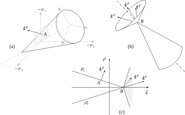
Fig. 7.2-5. Flow rule of Drucker-Prager model

Example

*Material, TYPE=DruckerPrager, Name=concreteDP
 2E6, 0.18, 1E-5, 7850, StrainHardening   # E, nu, alpha, density, StrainHardening|IsotropicHardening
 4        # beta
 12.3     # coh,dcoh|cohFunc, 
 20       # af,daf|afFunc 
 20       # ap,dap|apFunc  

*Material Type=ConcreteDamage

Define concrete damage plasticity

*Material, Type=ConcreteDamage, Name=name
 E, nu, alpha, density
 fc, Dc, wc, 
 ft, Dt, wt, 
 a, Kc, ap,ecc 

First dataline

• E: elastic modulus (required)
• nu: Poisson’s ratio (optional, default 0.)
• alpha: themal expansion coefficient (optional, default 0.)
• density: density (optional, default 0.)

Second dataline

• fc,Dc,wc: compressive uniaxial yield function(required), damage function(option, default none), and recovery(optional, default 0.)

3rd dataline

• ft,Dt,wt: tensile uniaxial yield function(required), damage function(option, default none), and recovery(optional, default 0.)

4th dataline if necessary (parameters for yield surface and flow potential)

• a: parameter for yield surface related to biaxial stress condition (optional, default 0.14),
• Kc: parameter for yield surface related to triaxial stress condition (optional, default 2/3),
• ap: parameter for flow potential related to dilatency(optional, default 0.2)
• ecc: parameter for flow potential, the eccentricity(optional, default 0.1)

Example

*Function, Name=chard
 0., 20.
 0.001, 25.
 0.002, 25.

*Function, Name=thard
 0., 2.
 0.001, 1.
 0.002, 0.2. 

*Material, TYPE=ConcreteDamage, Name=concreteCD
 29188.6, 0.18, 2300, 1e-05  #  E, nu, alpha, density
 chard,  , 1  # fc, Dc, wc n thard,  , 1  # ft, Dt, wt
 0.12 , 0.666667, 0.2, 0.1  # a, Kc, ap, ecc

*Material Type=UConcrete

Define uniaxial concrete

*Material, Type=UConrete, Name=name 
  CEnvFunc, Plastic|Secant|CIEFunc, alpha, density, timeProp
  TEnvFunc, Plastic|Secant|TIEFunc 

First dataline

• CEnvFunc: Compressive envelope function (required)
• Plastic|Secant|CIEFunc: - Plastic unloading, Secant unloading, 또는 damage plastic unloading 시의 함수를 지정 (optional, default Plastic)
• alpha: themal expansion coefficient (optional, default 0.)
• density: density (optional, default 0.)
• timeProp: Combined viscosity material given by *Material, Type=UConcreteTime. (optional)

2rd dataline if necessary

• TEnvFunc: Tensile envelope function (optional)
• Plastic|Secant|TIEFunc: - Plastic unloading, Secant unloading, 또는 damage plastic unloading 시의 함수를 지정 (optional, default Secant)
• TIEFunc: Tensile unloading function iff Plasticity (optional)

UConctete 모델은 콘크리트의 압축측 제하와 재재하에서 발생하는 에너지 소산을 무시하여 간략화한 소성손상모델이다. 압축 및 인장측에 대해 독립적으로 파괴포락선이 정의되어야 하며, 제하/재제하(unloading/reloading)시 손상이 없는 소성모델(이하 plastic), 소성손상모델(이하 damage plastic), 소성탄성모델(이하 damage elastic)을 선택할 수 있다. 만약 소성손상모델을 적용하는 경우 마지막으로 경험한 변형률(\(\small\epsilon_{cun}\) 또는 \(\epsilon_{tun}\)에 대응하는 점 \(\small(\epsilon_{cun},\sigma_{cun})\) 또는 \(\small(\epsilon_{tun},\sigma_{tun})\)과 소성변형률함수에서 지정된 소성변형률( \(\small\epsilon_{cpl}\) 또는 \(\epsilon_{tpl}\)에 대응하는 점을 잇는 선분을 따라 제하 및 재재하가 이루어지므로 \(\small(\epsilon_{cpl},\sigma_{cun})\), \(\small(\epsilon_{tpl},\sigma_{tun})\)형태의 함수 지정이 필요하다.

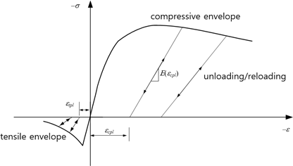
Fig. 7.2-6. Failure envelope, unloading/reloading of UConcrete

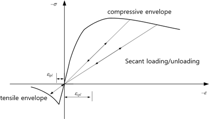
Fig. 7.2-7. Secant unloading/unloading of UConcrete

반복하중(cyclic loading) 조건에서는 소성변형률에 대응하는 항복값까지 탄성거동을 이후 파괴포락선을 따라 항복한다. Secant loading/unloading을 지정한 경우는 해당하는 비탄성변형률이 없다.

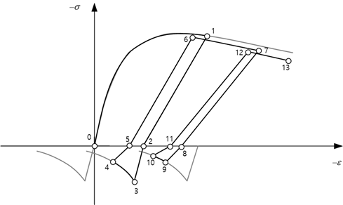
Fig. 7.2-8. Cyclic loading of UConcrete

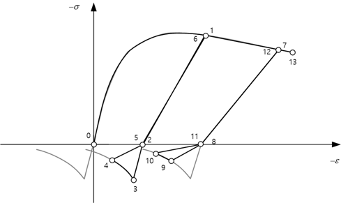
Fig. 7.2-9. Cyclic loading of Unconcret for tensile secant unloading

Example

*Function, Type=MPPCEnv, Name=MPP
 27, 25000, 0.002   # fco, Ec, eco, ecu, fcc, esp

*Function, Type=MPPCIE, Name=MPPIE
 MPP   # compressiveEnv, epeak 

*Function, Type=MaekawaTEnv, Name=Maekawa
 MPP, 3, 0.4  # compressiveEnv,ft, c

*Material, Type=UConcrete, Name=Mander
 MPP, MPPIE
 Maekawa,Secant   

*Material, Type=UConcrete, Name=Mander
 MPP
 Maekawa, Secant

*Material Type=USteel

Define uniaxial steel model based on Menegotto-Pinto model

*Material, Type=USteel, Name=name 
  E0, yield, E1,  R0,a1,a2, a3,a4, eu, alpha, density

First dataline

• E0: Initial tangent modulus (required)
• yield: yield stress ( required )
• E1: Second tangent modulus (optional, default 0.)
• __R0,a1,a2:__curvature parameters (optional, default 20, 0, 0)
• a3,a3: isotropic hardening parameters (optional, default 0, 1.)
• eu: ultimate strain (optional, default 0). If eu = 0., then ultimate strain is not checked.
• alpha: themal expansion coefficient (optional, default 0.)
• density: density (optional, default 0.)

USteel uses Menegotto-Pinto model with some modifications of partial reloading problem. It can be used for modeling rebar or prestressing steel.

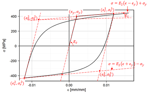
Fig. 7.2-10. Menegotto-Pinto Model

The recommended values of modeling rebar and 7-wire strand is given in the example.

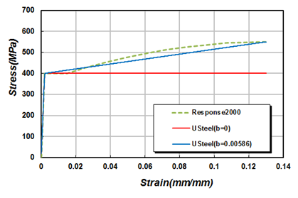
Fig. 7.2-11. Stress-strain curve of a weldable rebar with 400 MPa yield strength

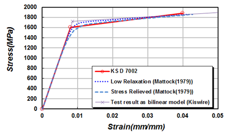
Fig. 7.2-12. Stress-strain curve of 7-wire strand with ultimate strength 1860 MPa

Example

# 400 MPa rebar without hardening
*Material, Type=USteel, Name=SD40
 200000,400, 0, 20,18.5,0.15, 0.01, 7, 0.08
#  E0, yield, E1, R0,a1,a2, a3,a4, eu, alpha, density

# 400 MPa weldable rebar without hardening
*Material, Type=USteel, Name=SD40W
 200000, 400, 0, 20,18.5,0.15, 0.01, 7, 0.13
#  E0, yield, E1, R0,a1,a2, a3,a4, eu, alpha, density

# 400 MPa rebar with hardening
*Material, Type=USteel, Name=SD40-U
 200000, 400, 0.01282*200000, 20,18.5,0.15, 0.01, 7, 0.08

# 400 MPa weldable rebar with hardening
*Material, Type=USteel, Name=SD40W-U
 200000, 400, 0.0586*200000, 20,18.5,0.15, 0.01, 7, 0.13

# Stress-relieved 7-wire strand with ultimate strength 1860 MPa 
*Material, Type=USteel, Name=STendon
 200000,  1652.891, 200000*0.03, 6, 0., 0., 0, 1, 0.0428

# Low relaxation 7-wire strand with ultimate strength 1860 MPa 
*Material, Type=USteel, Name=RTendon
 200000,  1694.915, 200000*0.025, 10,0.,0., 0, 1, 0.0415

*Material Type=GapHook

1축 gap-hook 재료를 지정

*Material, Type=GapHook, Name=name 
  kg,g, kh,h

First dataline

• kg,g: tangent and gap in compression part (optional, default 0.,0.)
• __kh,h:__tangent and hook tension part (optional,default 0.,0.)

GapHook 명령으로 tension only나 compression only 등으로 모델링할 수 있다. kg와 kh가 동시에 0이 될수 없다.

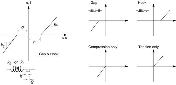
Fig. 7.2-135.GapHook Model

Example

*Material, Type=GapHook, Name=gaphook
 5E5, 0.1, 4E5, 0.2   # kg, g, kh, h

# tension only
*Material, Type=GapHook, Name=cable
 0, 0, 5E5   # kg, g, kh, h

# compression only
*Material, Type=GapHook, Name=contactSpring
 5E5   # kg, g, kh, h

*Material Type=Acoustic

Acoustic solid 요소용 acoustic material을 지정

*Material, Type=Acoustic, Name=name 
  bulk, density

First dataline

• bulk: Bulk modulus (required). If zero bulk moduls is given, the acoustic medium is assumed to be incompressible (Laplace equation is used)
• __density:__density (required)

Example

*Material, Type=Acoustic, Name=water
 2190E6, 1000

*Material Type=Porous

Porous solid 요소용 porous material을 지정

*Material, Type=Acoustic, Name=name 
  solidMat, wBulk, wDen, porosity, perm

First dataline

• solidMat: normal material for solid
• wBulk: bulk modulus of water (required)
• wDensity: water density(required)
• porosity: porosity (required)
• perm: permeability (required)

Example

*Material, Type=Porous, Name=water
 mat, 1000, 100, 0.1, 1000