8. 함수
함수는 *Function으로 지정한다. 고유이름을 가지며 이름은 중복하여 지정할 수 없다. *Function은 시간함수나 재료모델에서의 파괴포락선 함수 등으로 사용되는 함수이다.
*Function
Define function
*FUNCTION, TYPE=type, Name=name
  dataline...
Keyword line
- TYPE=type: type of function
- MultiLinear: Multi-linear function
- TimeSignal: Time signal. Multi-linear function with fixed step size
- String: function by mathematical expression
- HognestadCEnv: Hognestad concrete compressive envelope
- FIBCEnv: FIB concrete compressive envelope
- MPPCEnv: Mander-Pristley-Park concrete compressive envelope
- MPPCIE: Mander-Pristley-Park concrete compressive inelastic strain
- MaekawaTEnv: Maekawa concrete tensile envelope
- Name=name: function name
함수 관련 명령어는 \(\small y=f(x)\) 또는 \(\small y1=f1(x), y2=f2(x), ...\)형태의 함수를 정의한다. 함수는 재료 모델을 정의할 때 포락선을 정의하거나, 하중을 정의할 때 시간이력으로 사용된다. 함수는 자신만의 이름을 가지며 중복될 수 없다.
*Function, Type=MultiLinear
Multilinear function
*Function, Type=MultiLinear, Name=name
 x, y1, y2, ..., yn
 ...
First dataline and subsequent datalines
- x, y1, y2, ..., yn: (x,y1,y2,..., yn) 형태로 입력.
MultiLinear 함수는 y1(x), y2(x), ... 함수를 (x, y1(x), y2(x), ..., yn(x)) 형태로 정의한다.
Example
*Function, Type=MultiLinear, Name=func1
 0., 45.3
 2.802903E-3, 86.4
 7.26864E-5, 122.5

*Function, Type=MultiLinear, Name=func2
 0., 45.3, 12.3
 2.802903E-3, 86.4, 5.1
 7.26864E-5, 122.5, 3.1
*Function, Type=TimeSignal
Time signal. Multi-linear function with fixed step size
*Function, Type=TimeSignal, Name=name
 dtime, ntime
 file, nseries, scaleFactor, skipRows
 ...
First dataline
- dtime: time step (required).
- ntime: number of time data (optional). 읽힌 데이터의 row 수가 ntime보다 많은 경우 무시되고, 작은 경우는 0으로 채워짐. 만약 ntime이 주어지지 않으면 시계열 중 가장 긴 개수로 설정됨. 나머 시계열은 자신의 길이보다 긴 경우 ntime까지 0으로 채워짐.
Second dataline and subsequent datalines
- file: 읽을 파일(required). 콤마, 공백 등으로 구분된 텍스트파일 또는 npy 파일
- nseries: 파일 내의 시계열 개수(optional, default 1). npy 파일인 경우 column 개수가 동일해야 함.
- scale: scale Factor(optional, default 1)
- skipRows: 파일 앞부분 무시하는 줄 수(optional, default 0). npy 파일에서는 무시됨.
시간이력을 나타내는 데 적합한 TimeSignal 함수는 고정 간격의 x 값을 갖는 multi linear 함수로 이해할 수 있다. 파일의 데이터는 공백문자(콜론, 스페이스, 탭, 줄바꿈)로 구분되어 읽힌다. 각 파일에서 nseries개의 시계열 데이터를 구성한다. nseries 개의 데이터를 ntime 개 만큼 읽어 들이다. 만약 파일에서 데이터 수가 부족한 경우 0으로 채우게 된다. 시각 0에서는 값이 0으로 가정되며, 데이터로 주어진 첫 번째 값은 시각 dt에서의 값이다. 최종값은 시각 ntime*dt에서의 값이다.
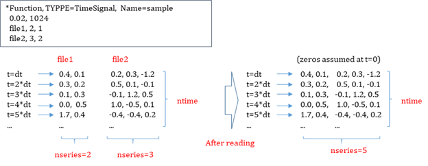
Fig. 8.2-1. TimeSignal function
시간데이터 파일에서 # 이후 내용은 무시한다(comment)
Example
*Function, TYPE=TimeSignal, Name=EqAcc
 0.02, 1024              # dt, ntime
 elcenX.dat, 1, 3.01      # file, nseries, scaleFactor
 elcenYZ.dat, 2, 3.01, 4      # dataFile, nseries, scaleFactor, skipRows
*Function, Type=String
Define function by mathematical expression
*Function, Type=STRING, Name=name
  expreesion, min,max
First dataline
- expression: Expression with x independent variable, such as "sin(x)+1". Note tha white space is not allowed.
- min,max: minimun and maximun range. Zero function value is assumed beyond the givne range. If Range keyword is not given, no range check is performed
csin(x), cos(x), tan(x), acos(x), atan(x), cosh(x), sinh(x), tanh(x), fabs(x), exp(x), log(x), log10(x), sqrt(x), step(x), sgn(x), and pow(x,n).
Example
*Function, Type=String Name=Half-sine
 sin(2*pi/1.2*x), 0., 0.6
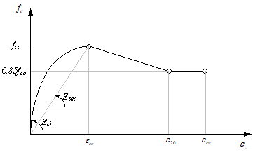
*Function, Type=HognestadCEnv
Hognestad의 콘크리트 재하곡선(compressive envelope)을 정의한다.
*Function, Type=HognestadCEnv, Name=name
  fco, Ec, ec20, ecu
First dataline
- fco: compressive strength (requied)
- Ec: initial tangent modulus (required)
- ec20: straint at 0.85fcm concrete stress of of descending branch(optional, default 0.003)
- ecu: ultimate strain (optional, always set to max(ec20, ecu) )
Hognestad’s cmpressive envelope of concrete given as
where, \(\small\epsilon_{20}\) coressponding to \(\small f_{co}\) is given as
ccccccccc
Example
*Function, Type=HognestadCEnv, Name=HognestadTest1
 25., 23500.

*Function, Type=HognestadCEnv, Name=HognestadTest2
 25., 23500., 0.0031, 0.0032

*Function, Type=HognestadCEnv, Name=HognestadTest3
 25., 23500., 0.0032
*Function, Type=ParabolaCEnv
EC2와 KDS에서 정의하고 있는 단면 설계를 위한 응력-변형률 재하곡선(compressive envelope)을 정의한다.
*Function, Type=ParabolaCEnv, Name=name
  fco, n, eco, ecu
First dataline
- fco: design compressive strength, (requied)
- n: shape factor (required)
- eco: peak strain (optional, 0.002)
- ecu: ultimate strain (optional, always set to max(eco, ecu) )
The curve given as
where, \(\small f_{co} = \phi_c (0.85f_{ck})\), \(\small\phi_c = 0.65\) for ultimate limit state. \(\small\phi_c = 1\) for extreme limit state.
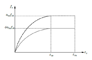
Fig. 8.2-3. ParabolaCEnv function
The elastic modulus, which is the tangent slope, is calculated as follows.
Example
*Function, Type=ParabolaCEnv, Name=ParabolaTest1
  0.85*27, 1.8, 0.00203, 0.0033     #  fco, n, eco, ecu
*Function, Type=FIBCEnv
CEB/FIB MC90의 콘크리트 재하곡선(compressive envelope)을 정의한다.
*Function, Type=FIBCEnv, Name=name
 fcm, Ec, eco
First dataline
- fcm: compressive strength (requied)
- Ec: initial tangent modulus (required)
- eco: strain at peak concrete strength (optional, default automatically computed)
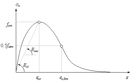
Fig. 8.2-4. Compressive Failure Envelope of EB-FIP MC90
Example
*Function, Type=FIBCEnv, Name=FIBCEnvTest1
 25., 23500.   #  fcm, Ec, eco

*Function, Type=FIBCEnv, Name=FIBCEnvTest2
 25., 23500., 0.002     #  fcm, Ec, eco
*Function, Type=MPPCEnv
Mander, Priestly, Park의 콘크리트 재하곡선(compressive envelope)을 정의한다.
*Function, Type=MPPCEnv Name=name
  fco, Ec, eco, ecu, fcc, esp
First dataline
- fco: unconfined compressive strength (requied)
- Ec: initial tangent modulus (required)
- eco: strain at peak strength of unconfied concrete (optional, default 0.002)
- ecu: ultimate strain (optional, default 2*eco)
- fcc: confined compressive strength. (optional, default fco)
- esp: spalling strain (optional, default ecu). The straight line from to is assumed, if and only if is greater than ,
The Mander-Priestly-Park model can define both the confined and unconfined concrete model.
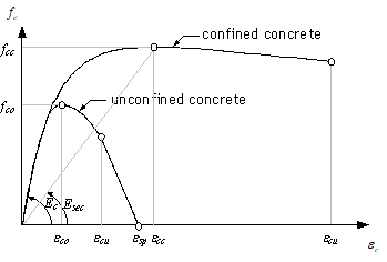
Fig. 8.2-5. Compressive Failure Envelope of Mander, Priestley, Park’s Concrete Model
Example
*Function, Type=MPPCEnv, Name=MPPCEnvTest1
 25., 23500.   #   fco, Ec, eco, ecu, fcc, esp

*Function, Type=MPPCEnv, Name=MPPCEnvTest2
 25., 23500., 0.002, 0.004, 40., 0.006    #   fco, Ec, eco, ecu, fcc, esp
*Function, Type=MPPCIE
Mander, Priestly, Park의 콘크리트 비탄성 변형률을 정의한다.
*Function, Type=MPPCIE Name=cover
  compressiveEnv, epeak
First dataline
- compressiveEnv: Compressive envelope function
- epeak: strain at peak concrete stength(optional, default 0.002). If the given compressiveEnv is a type of MPPCEnv, Hognestad, and CEBFIB, epeak is neglected(automatically computed),.
Although this function deefines the inelastic strain by the Mander-Priestly-Park model, it can be used with the abitary compressive envelope function
Example
*Function, Type=MPPCEnv, Name=concC
 25., 23500.

*Function, Type=MPPCIE, Name=concCI
 concC
*Function, Type=MaekawaTEnv
Maekawa’ concrete tensile envelope
*Function, Type=MaekawaTEnv Name=coverTension
  compressiveEnv,ft, c
First dataline
- compressiveEnv: Compressive envelope function(required)
- ft: tensile strength(required)
- c: parameter for Maekawa model (optional, default 0.4)
Maekawa 등(2002)는 보통콘크리트와 인장경화를 고려한 철근콘크리트에 대한 모델에 대한 인장연화곡선을 다음과 같은 동일한 수식으로 제안하였다.
위에서 는 곡선형상을 결정하는 인자이다. 보통콘크리트로 사용할 때는 파괴에너지와 요소특성길이에 따라 다음 식으로부터 결정해야 한다.
철근콘크리트에서는 매개변수 분석을 통해 이형철근의 경우 0.4, 용접강선망(welded wire mesh)의 경우 0.2를 제시하고 있다. 그림 8.2-5는 대표적인 결과를 나타낸 것이다.
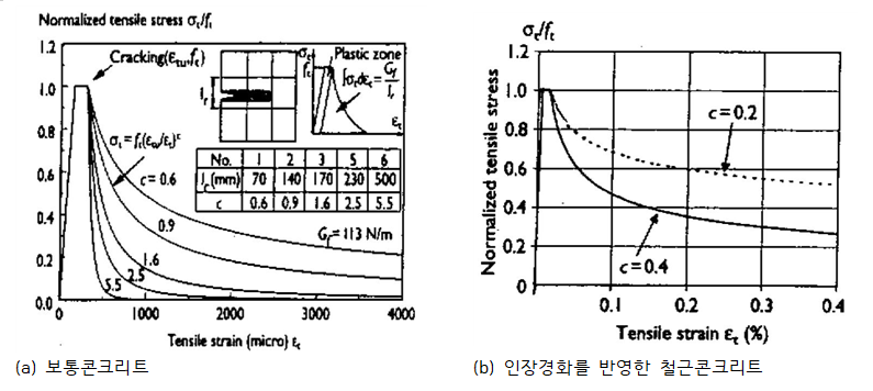
Fig. 8.2-6. Tensile Failure Envelope of Maekawa model
Example
*Function, Type=MPPCEnv, Name=concC
 25, 23500.

*Function, Type=MaekawaTEnv, Name=concT
 concC, 3