E.6 Acoustic Solid Element

E.6.1 Impulsive Natural Frequencies in a Rigid Rectangular Tank

가로, 세로, 높이가 \(\small L_{x},\ L_{y},\ H\)인 강체 직사각 탱크에 담긴 압축성 유체에서, 상면은 압력이 0인 조건을 나머지 면은 플럭스가 0인 조건을 부과하면, 다음과 같은 고유치를 해석적으로 유도할 수 있다.

\[ \small \begin{array}{r} \omega_{lmn} = c\sqrt{\alpha_{l}^{2} + \beta_{m}^{2} + \gamma_{n}^{2}}\tag{E.6.1} \end{array} \]

where

\(\small c\) is acoustic wave velocity, 1480 m/s/s if water

\(\small \alpha_{l} = \frac{l\pi}{L_{x}},\ \beta_{m} = \frac{m\pi}{L_{y}},\gamma_{n} = \frac{(2n - 1)\pi}{2H}\)

\(\small l,m = 0,1,2,\ldots,\ \ n = 1,2,\ldots\)

가로, 세로, 높이가 40m, 30m, 20m인 직사각 물탱크를 대상으로 3차원 조건에 대해 세가지가 메쉬에 대해 고유진동수 해석을 수행하고 그 결과를 해석해와 비교하였다.

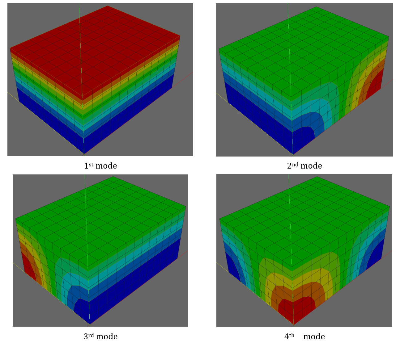
Figure E.6.1 Contour Plot of Mode Shapes

Table E.6.1 Natural Frequencies of 3D Rigid Rectangular Tank

l	m	n	Analytic solution					Numerical solution
l	m	n	alpha	beta	gamma	wlnm	frq	8x4	12x6	16x8	16x12-P6	16x12-P8	16x12-P8+T4
0	1	0	0	0	0.07854	116.2389282	18.5000	18.6191	18.5529	18.5297	18.5242	18.5259
1	0	0	0.07854	0	0	164.3866687	26.1630	26.3314	26.2377	26.2054	26.1758	26.1755
2	0	0	0.15708	0	0	193.7315497	30.8333	31.131	30.9654	30.9076	30.9008	31.0321
0	2	0	0	0.15708	0	225.2967575	35.9631	36.2474	36.0653	35.9496	35.9369	36.3651
1	1	0	0.07854	0.07854	0	259.918145	41.3673	42.2775	41.7704	41.5937	41.5099	42.0162
0	0	1	0	0	0.07854	302.6185304	48.1632	49.0003	48.5738	48.3938	48.6972	49.1273
2	1	0	0.15708	0.07854	0	343.0194616	53.1680	54.3603	53.2028	53.2827	53.4984
1	2	0	0.07854	0.15708	0	348.7167845	55.0038	57.3957	56.7676	56.3055	56.1504	56.2974
0	1	1	0	0.07854	0.07854	350.865724	55.8415	56.9935	56.3651	56.1431	56.1939	56.1939
1	1	1	0.07854	0.07854	0.07854	357.5797658	58.5021	61.6157	59.8217	59.0764	59.5911	59.91
3	0	0	0.235619	0	0	367.5797658	58.5021	61.6157	59.8217	59.0764	59.5911	59.91
2	2	0	0.15708	0.15708	0	381.8089616	60.7346	63.6522	61.4999	61.5399	62.0894
3	1	0	0.235619	0.10472	0.07854	398.9176709	63.49972	66.4765	64.81	64.2307	64.6278	65.3594
1	3	0	0.07854	0.235619	0.10472	399.9176709	63.49972	66.4765	64.81	64.2307	64.6278	65.3594
2	1	2	0.15708	0.20944	0.07854	404.5233462	64.3819	66.7128	65.4134	64.9680	65.1404	65.5128
2	0	2	0.15708	0	0.235619	419.1054158	66.7027	69.9335	68.1335	67.5055	67.0949	69.9077

가로, 높이가 40m, 20m인 직사각 물탱크를 대상으로 2차원 조건에 대해 세가지 메쉬에 대해 고유진동수 해석을 수행하고 그 결과를 해석해와 비교하였다. 해석해에서는 항상 \(\small m = 0\)인 경우이다.

Table E.6.2 Natural Frequencies of 2D Rigid Rectangular Tank

l	m	n	Analytic solution					Numerical solution
l	m	n	alpha	beta	gamma	wlnm	frq	8x4	12x6	16x8	16x8-T
1	0	0	0	0	0.07854	116.2389282	18.5000	18.6191	18.5529	18.5297	18.5296
1	0	1	0.07854	0	0.07854	164.3866687	26.1630	26.3314	26.2377	26.2054	26.2881
2	0	1	0.15708	0	0.07854	259.918145	41.3673	42.2775	41.7704	41.5937	41.8000
0	2	0	0	0.235619	0	348.7167845	55.0000	58.7365	56.9352	56.3055	56.2984
3	0	0	0.235619	0	0.07854	367.5797658	58.5021	61.617	59.8217	59.2761	59.5851
2	1	0	0.07854	0.235619	0	419.1054158	66.7027	69.934	68.6325	67.6535	68.6724
4	0	0	0.314159	0	0.07854	479.2653787	76.2775	83.066	79.6017	78.1423	78.3488
3	0	2	0.235619	0	0.235619	493.1600601	78.4889	83.694	80.5185	79.6281	82.91

Input File

tank2d-8x4.inp : 2 dimensional rectangular tank, 8x4 elements, AC2D4
tank2d-12x6.inp : 2 dimensional rectangular tank, 12x6 elements, AC2D4
tank2d-16x8.inp : 2 dimensional rectangular tank, 16x8 elements, AC2D4
tank2d-16x8-T3.inp : 2 dimensional rectangular tank, 16x8*2 elements, AC2D3
tank3d-8x6x4.inp : 3 dimensional rectangular tank, 8x6x4 elements, AC3D8
tank3d-12x9x6.inp : 3 dimensional rectangular tank, 12x9x6 elements, AC3D8
tank3d-16x12x8.inp : 3 dimensional rectangular tank, 16*12*8 elements, AC3D8
tank3d-16x12x8-T4.inp : 3 dimensional rectangular tank, 16*12*8*6 elements, AC3D4
tank3d-16x12x8-P6.inp : 3 dimensional rectangular tank, 16*12*8*2 elements, AC3D6

E.6.2 Sloshing Natural Frequencies in a Rigid Rectangular Tank

비압축성 유체를 가정하는 경우, 직사각 탱크에서 유체 표면의 출렁임에 대한 고유진동수를 해석적으로 유도할 수 있다(Lamb, 1945)

\[ \small \begin{array}{r} \omega_{mn} = \sqrt{gk_{mn}\tanh\left( k_{mn}H \right)}\tag{E.6.2} \end{array} \]

where

\[ \small \begin{array}{r} \ k_{mn} = \sqrt{\alpha_{m}^{2} + \beta_{n}^{2}},\ \ \alpha_{m} = \frac{m\pi}{L_{x}},\ \ \beta_{n} = \frac{n\pi}{L_{y}},\ where\ \ l,m = 0,1,2,\ldots,\ \ n = 1,2,\ldots\tag{E.6.3} \end{array} \]

Housner(1957)은 Fundamental frequency에대한 근사식을 다음과 같이 제안하였다.

\[ \small \begin{array}{r} \omega^{2} = \frac{g}{L/2}\sqrt{\frac{5}{2}}\tanh\left( \sqrt{\frac{5}{2}}\frac{H}{L/2}\ \right)\tag{E.6.4} \end{array} \]

여기에서 L은 excitation 방향의 길이이다.

Table E.6.3 Natural Frequencies of Sloshing Modes in 3D Rigid Rectangular Tank

m	n	kmn	f	Numerical solution
m	n	kmn	f	10x30x6	20x60x11	20x60x11-P6	20x60x11	20x60x11-T4
0	0	0.000	0.000	0	0	0	0
0	1	0.053	0.084	0.084416	0.084368	0.084368	0.084372
0	2	0.107	0.149	0.149068	0.148796	0.148783	0.148874
1	0	0.160	0.194	0.195056	0.19439	0.194329	0.194702
0	3	0.160	0.194	0.195056	0.19439	0.194343	0.195071
1	1	0.169	0.200	0.201226	0.200551	0.200536	0.201349
1	2	0.193	0.216	0.216947	0.216181	0.216238	0.217327
0	4	0.214	0.229	0.230264	0.229004	0.228874	0.229771
1	3	0.227	0.236	0.237313	0.236266	0.236372	0.237929
0	5	0.267	0.257	0.259196	0.257612	0.257536	0.258952
1	4	0.267	0.257	0.259909	0.257787	0.257734	0.260181
1	5	0.312	0.278	0.281321	0.278901	0.278968	0.281839
0	6	0.321	0.282	0.286557	0.283247	0.282861	0.285658
2	0	0.321	0.282	0.286557	0.283247	0.282862	0.287921
2	1	0.325	0.284	0.28854	0.285216	0.284879	0.290092
2	2	0.338	0.290	0.294289	0.290893	0.290692	0.296245

Table E.6.4 Natural Frequencies of Sloshing Modes in 2D Rigid Rectangular Tank

m	km	f	Numerical solution
m	km	f	30x6	60x11	60x11-T
0	0.000	0.000	0	0	0
1	0.053	0.084	0.084416	0.084368	0.084372
2	0.107	0.149	0.149068	0.148796	0.148875
3	0.160	0.194	0.195056	0.19439	0.194722
4	0.214	0.229	0.230264	0.229004	0.229799
5	0.267	0.257	0.259909	0.257787	0.259258
6	0.321	0.282	0.286557	0.283247	0.285611
7	0.374	0.305	0.311438	0.306572	0.310062
8	0.427	0.326	0.335203	0.323875	0.333244
9	0.481	0.346	0.358247	0.349017	0.355533
10	0.534	0.364	0.380845	0.368738	0.377183
11	0.588	0.382	0.403204	0.387712	0.398377

Input File

sloshing2d-30x6.inp : 2 dimensional rectangluar tank, 30*6 elements, AC2D4
sloshing2d-60x11.inp : 2 dimensional rectangluar tank, 60*11 elements, AC2D4
sloshing2d-60x11-T3.inp : 2 dimensional rectangluar tank, 60*11*2 elements, AC2D3
sloshing3d-10x30x6.inp : 3 dimensional rectangluar tank, 10*30*6 elements, AC3D8
sloshing3d-20x60x11.inp : 3 dimensional rectangluar tank, 20*60*11 elements, AC3D8
sloshing3d-20x60x11-T4.inp : 3 dimensional rectangluar tank, 20*60*11*6 elements, AC3D4
sloshing3d-20x60x11-P6.inp : 3 dimensional rectangluar tank, 20*60*11*6 elements, AC3D6

E.6.3 Natual Frequencies in a Rigid Cylinderical Tank

원통형 탱크를 대상으로 여러 가지 고유진동수를 계산하였다. Sloshing에 대한 정해는 다음과 같다.

(1) Veletos(1984)는 다음과 같은 식을 제안하였다.

\[ \small \begin{array}{r} \omega_{j}^{2} = \frac{\lambda_{j}g}{R}\tanh\left( \lambda_{j}\frac{H}{R}\ \right)\tag{E.6.5} \end{array} \]

여기에서 \(\small \lambda_{j}\)는 \(\small \frac{dJ_{1}(x)}{dx} = 0\)의 해이며, 저차 3개 값은 \(\small \lambda_{1} = 1.8411837813406593\), \(\small \lambda_{2} = 5.331442773525033\), \(\small \lambda_{3} = 8.536316366346286\) 이다.

(2) Housner(1957)은 Sloshing에 대한 Fundamental frequency에대한 근사식을 다음과 같이 제안하였다.

\[ \small \begin{array}{r} \omega^{2} = \frac{g}{R}\sqrt{\frac{27}{8}}\ \tanh\left( \sqrt{\frac{27}{8}}\frac{H}{R}\ \right)\tag{E.6.6} \end{array} \]

Sloshing frequency는 모두 incompressible water를 가정한 것이다. 한편 압축성을 고려할 경우 Impulsive 성분에 대한 정해는 직사각형과 같다(Lx = Ly = 2R)

wide 및 tall cylinder에 대해 해를 비교하였다. Wide Cylinder는 R = 18.3 m, H = 12.2 m이고, tall Cylinder는 R=10, H =30이다. 메쉬는 각각 2종을 준비하였으며 fundamental frquency를 비교한다.

Table E.6.5 Sloshing Freqencies of wideCylinder Model

Numerical Solution		Analytic Solution
Model	Natural Frequency	Analytic Solution
wideCylinderIncomp-15x10	0.145258 Hz	0.145075 Hz(Veletsos), 0.144846 Hz((Housner)
wideCylinder-15x10	0.145256 Hz
wideCylinderIncomp-30x15	0.14516 Hz
wideCylinder-30x15	0.145158 Hz

Table E.6.6 Impulsive Frequencies of wideCylinder Model

Numerical Solution		Analytic Solution
Model	Natural Frequency	Analytic Solution
wideCylinder-15x10	30.3591 Hz	30.3279 Hz
wideCylinder-30x15	30.3417 Hz	30.3279 Hz

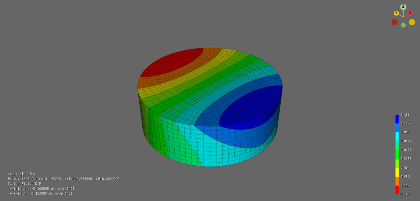
Figure E.6.2 Sloshing Mode of wideCylinder-20.x10

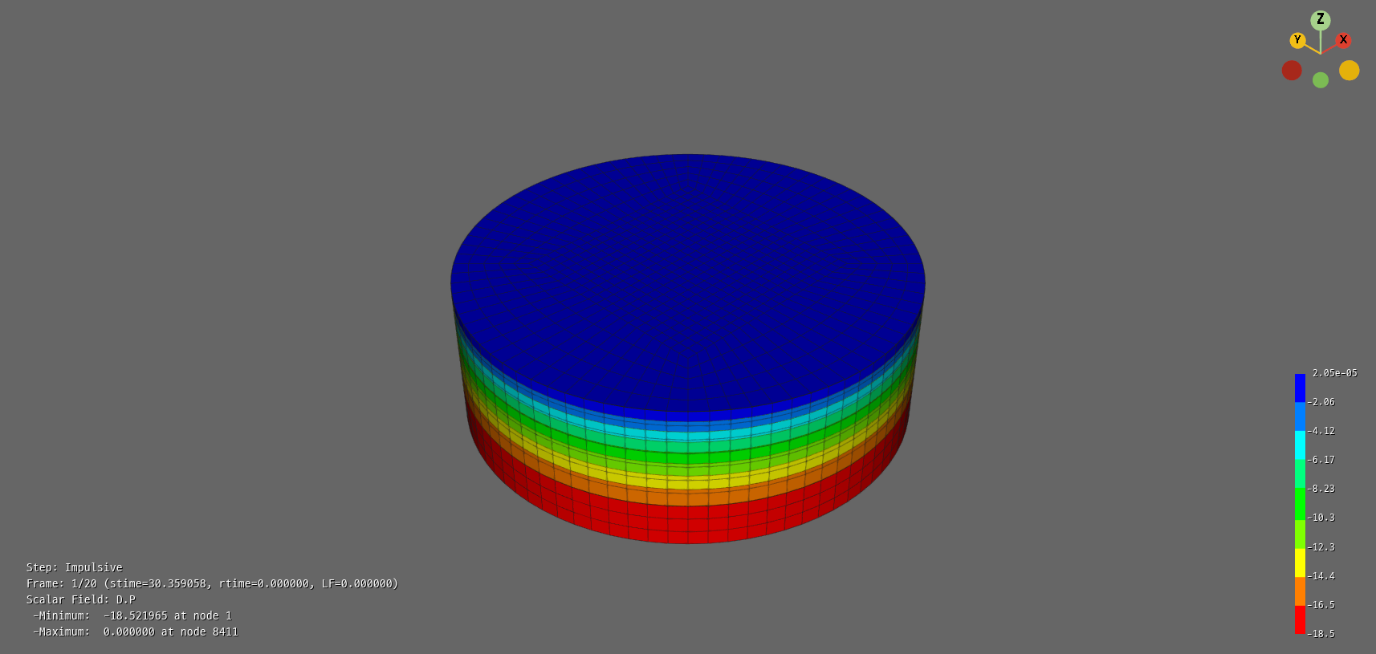
Figure E.6.3 Impulsive Mode of wideCylinder-20.x10

Table E.6.7 Solshing Freuencies of tallCylinder Model

Numerical Solution		Analytic Solution
Model	Natural Frequency	Analytic Solution
tallCylinderIncomp-10x10	0.21567 Hz	0.21389 Hz(Veletsos), 0.213656 Hz((Housner)
tallCylinder-10x10	0.215668 Hz
tallCylinderIncomp-15x15	0.21567 Hz
tallCylinder-15x15	0.215668 Hz

Table E.6.8 Impulsive Frequencies of tallCylinder Model

Numerical Solution		Analytic Solution
Model	Natural Frequency	Analytic Solution
tallCylinder-10x10	12.346 Hz	12.3333 Hz
tallCylinder-15x15	12.346 Hz	12.3333 Hz

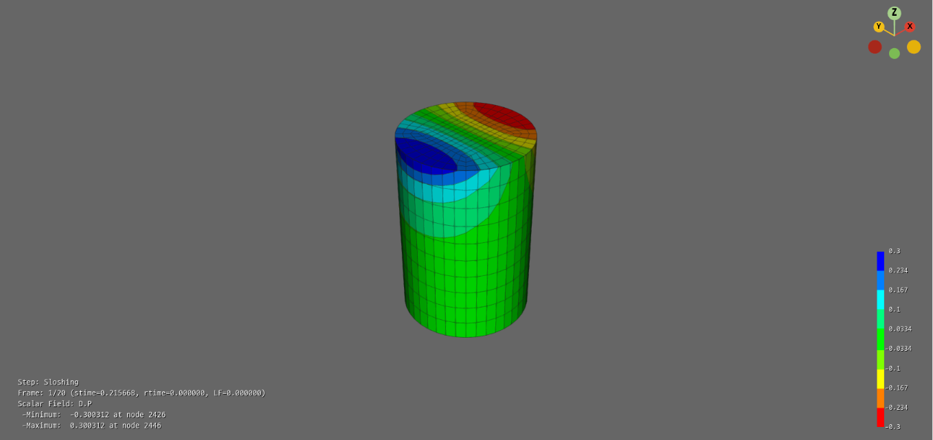
Figure E.6.4 Sloshing Mode of tallCylinder-10.x10

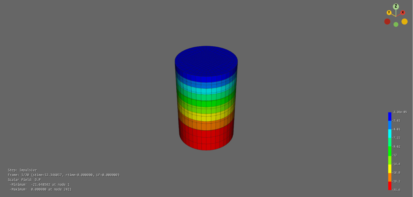
Figure E.6.5 Impulsive Mode of tallCylinder-10.x10

Input File

wideCylinder-20x10.inp : Wide Cylinder with 20*10 elements
wideCylinderIncomp-20x10.inp : Wide Cylinder with 20*10 elements, Incompressible Water
wideCylinder-30x15.inp : Wide Cylinder with 30*15 elements
wideCylinderIncomp-30x15.inp : Wide Cylinder with 30*15 elements, Incompressible Water
tallCylinder-10x10.inp : Tall Cylinder with 10*10 elements
tallCylinderIncomp-10x10.inp : Tall Cylinder with 10*10 elements, Incompressible Water
tallCylinder-15x15.inp : Tall Cylinder with 15*15 elements
tallCylinderIncomp-15x15.inp : Tall Cylinder with 15*15 elements, Incompressible Water

References

Lamb, H. (1945) Hydrodynamics, 6^th Edition, Dover Publications.
Veletos, A.S.(1984), Seismic reesponse and design of liquid storage tanks, Guidelines for the seismic design of oil and gas pipeline systems, ASCE
Housner, G. W. (1957). Dynamic pressures on accelerated fluid containers. Bulletin of the seismological society of America, 47(1), 15-35.